History of Normal Distribution

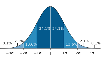
The origin of normal distribution can be traced to a French mathematician Abraham de Moivre. He had scientific interest in gambling and often acted as a consultant to gamblers to determine probabilities. De Moivre allegedly was studying the probability distribution of coin flips. He was trying to come up with a mathematical expression such as finding a probability of 60 or more tails out of one hundred coin flips. As an answer to this question he derived a bell shaped distribution which is commonly referred as the normal curve.
This was a crucial observation as a large number of phenomena follow approximately normal distribution. For example, such variables (phenomena) as height, weight and strength are characterized with normal distribution. That’s why it is possible to determine one’s weight or height standing compared to others using z score tables. A Belgian astronomer - Lambert Quetelet, was the first one who noticed the link between weight and height distribution and the normal curve.
This was a crucial observation as a large number of phenomena follow approximately normal distribution. For example, such variables (phenomena) as height, weight and strength are characterized with normal distribution. That’s why it is possible to determine one’s weight or height standing compared to others using z score tables. A Belgian astronomer - Lambert Quetelet, was the first one who noticed the link between weight and height distribution and the normal curve.

Initially the normal curve was used to analyze the errors of measurement in astronomical observations. These errors happened due to instrument imprecision and observers’ built-in bias.
It was Galileo who saw that errors were symmetric. He also observed that smaller errors were characterized by higher frequency. This gave an impetus to a chain of hypotheses about error distribution. However, it was only in nineteenth century that it was noted that these errors were normally distributed. Two mathematicians Adrian and Gauss developed formula for normal distribution independent of each other. Formula demonstrated that errors were well approximated by the normal curve.
It is worth noting that the same distribution was discovered by Laplace in late 18th century, when he developed very influential central limit theorem. According to this theorem, a

distribution of sample means (even if drawn from a non-normal distribution) follows the normal distribution. The larger the sample, the more the distribution approximates normal.
Normal distribution and related z score calculation have a wide application in a large number of fields ranging from social sciences to medicine. Z score is a useful standardized value which allows comparison among groups of people based on weight, height, test results, income and many other variables. If you need to find a z score use a z table here.
Normal distribution and related z score calculation have a wide application in a large number of fields ranging from social sciences to medicine. Z score is a useful standardized value which allows comparison among groups of people based on weight, height, test results, income and many other variables. If you need to find a z score use a z table here.